It is a strange year to try to judge the play of the Pittsburgh Steelers’ offensive line.
Quarterback Ben Roethlisberger currently leads the league in pass attempts. And he has only been sacked 12 times. That equates to a league-best 2.1-percent sack rate.
That should, under normal circumstances, speak incredibly highly of an offensive line.
But Roethlisberger is also getting rid of the ball at the record-setting average time of 2.15 seconds. The Steelers’ offensive line could be as porous as swiss cheese and defenses still would have difficulty registering sacks in that time frame.
On the other hand, the running game this season has continued to be lacking. James Conner currently has 663 yards on the ground, averaging just 60.3 per game. Benny Snell Jr. has 358 yards for an average of 25.6 per game. Further, the rushing attack has failed to post a 100-yard game eight different times this season.
So, yes: the Steelers’ offensive line is difficult to gauge. Moreover, offensive line play in general is underserved by statistics.
In order to further understand the play of this year’s offensive line, I turned to the work of Brian Burke who – prior to moving over to ESPN – hosted his own blog where he showcased his analytics work. Way back in November 2014, he wrote a post that detailed his process in determining and, in the end, valuing an offensive line’s performance.
Doing so is understandably difficult. First, as Burke points out, an offensive line’s performance on the field is often characterized by the overall “absence” of stats.
The less sacks, short yardage plays, tackles for loss, and quarterback scrambles – for example – the better. But how can the performance of an offensive line be quantified based on statistics that are absent?
That leads to the second issue in the difficulty providing valuation to offensive lines. Again, as pointed out by Burke, an offensive line’s role is, at its core, defensive. The linemen must protect. And that ultimately means that the less success the defensive line has, the more success the offensive line has.
So, again: how to you quantify that with numbers?
To do so, Burke devised a rather ingenious method that is simple at its core: to measure the value of an offensive line’s play, you must determine the impact in which the opposing defensive line had on the game.
In his 2014 work on the topic, Burke used quarterback sacks, tackles for losses and/or short gains, tipped passes, and quarterback hits to provide a quantifiable valuation to a defensive line to then calculate the valuation of the opposing offensive line.
In other words, while the metrics that define an offensive line’s ability may be “absent,” many of the factors that determine a defensive line’s valuation are statistically recorded.
Building upon Burke’s previous work, I wanted to run the same sort of study on the Steelers’ offensive line using the publicly available data in the nflfastR project.
To determine the impact of a defensive line’s play, I used the following standard metrics:
- Sacks
- Tackles for loss
- Yards gained less than/equal to 2
- Forcing a QB scramble
- Air yards less than/equal to 2
As mentioned, all five of those metrics are readily available and recorded in the play-by-play provided by nflfastR. However, to provide as much context to a defensive line’s impact as possible, I created several other metrics to add to the equation:
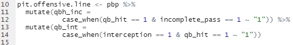
In the first mutation above, I am adding an additional filter for those play where Roethlisberger was hit, but not sacked, and the result of the play was an incomplete pass. The inclusion of this allows for the addition of defensive line pressure effecting the timing and/or accuracy of Roethlisberger’s throws.
The second mutation also registers QB hits, but searches for those situations where the result of the play is an interception. The same as above, the creation of this new metric allows for further inclusion of defensive line pressure altering the winning probability conditions of the game.
Once the mutations are created and added to the play-by-play data frame, you can run the numbers and get the results for each week of the season. However, as Burke points out, that simply does not provide enough information to draw a meaningful conclusion because even the most elite offensive lines cannot avoid negative-pointed plays. To correct this issue, the same information run to gather Pittsburgh’s week-by-week WPA for its offensive line must be conducted league-wide and then the difference calculated.
Doing so results in the following charts for Pittsburgh’s 2020 offensive line:

Because I compared the Steelers week-by-week WPA for its offensive line against the rest of the league, the chart means that the Steelers’ offensive line provided .25 percent more WPA in week one than the rest of the NFL. In week ten, against the Cincinnati Bengals, the Steelers’ offensive line had a season high WPA, adding a 12-percent chance to winning the game compared to all the other offensive lines in that single week.
On the other hand, the offensive line has struggled the last two weeks very much. In week 14 against the Buffalo Bills, the play of the offensive line cost the Steelers a 17-percent chance at winning. The second game with the Bengals was not much better, with the offensive line costing Pittsburgh a 14-percent chance at winning.
That said, this method is not perfect. As Burke mentioned, the play of quarterbacks and running backs are still independent from the play of the offensive line. But it does provide a somewhat reliable avenue in which to independently isolate the play of the offensive line. My plan is to continue to tinker with this model, as the mutate function in the R programming language – as mentioned above – provides significant ability to create new metrics, based on very specific scenarios, that will help in further isolating the valuation of offensive line play.