Part 2: Offensive Performance
Midway through the 2019 season Jameis Winston was given the distinct honor of “Turnover Machine” by Kevin Seifert at ESPN. At the time, he had committed 16 turnovers in only 8 games. By the end of the year, according to Pro Football Reference he ended up throwing the same number of pick sixes (7) – more than double the second place Andy Dalton (3) – as the Steelers had offensive rushing touchdowns in 2019. To his credit, he was tied for most passing attempts and did produce a lot of positive plays, leading the league in passing by over 200 yards and second in touchdowns thrown.
Importantly, while many metrics rate Winston as more of an average value at quarterback like passer rating (26th) and adjusted net yards per passing attempt (18th). It is valuable to ask why Winston’s scoring wasn’t corrected for the negative plays he committed. In a broader sense, teams offensively are often also only statistically presented to fans like kickers, where the rankings don’t combine the good and bad plays they have for context. For example, the Buccaneers were the 3rd highest scoring offense in 2019, putting up ~28.6 points per game and 3rd most total yards (~400 yards per game) according to Pro Football Reference. Subtracting only the from the pick sixes (which were a clear outlier league wide) by Winston, the Bucs would be outside of the top 5 (7th with ~25.1 points per game).
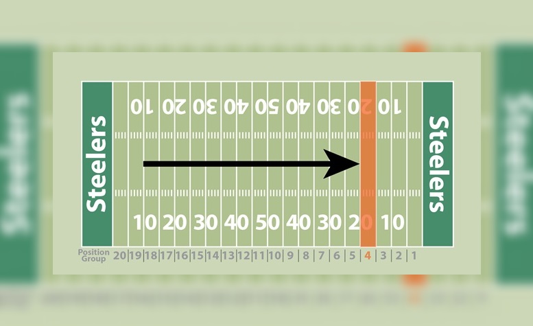
In this post, we will dig into one way to try to better contextualize offensive performance to understand how rankings of teams changes by adjusting the underlying scoring data. Taking the same approach from the previous post, we will be looking at correcting scoring based on field position groupings (explained in the previous post and visualized below).

As this post will have a few more calculations to correct the scoring than kickers, I will first present the approach in a simplified way, then at the bottom go through the calculation in more detail. If you are interested in that first, you can feel free to scroll down before reading the next portion.
In the previous post, I brought up how a Duck Hodges interception in the Steelers-Bills game last year resulted in putting the Steelers defense in a position where they were doomed to give up at least a field goal. Looking at it in the other way, the Steelers led the league last year in takeaways, giving the offense several positions with positive opportunities to score. In the kicking post, kicking points were corrected based on how difficult the kick distance was. Here, offensive scoring and outcomes will be corrected by where the team started off the drive.
Taking all the drive data from Pro Football reference, I included only plays outside the final 2 minutes of each half, overtime, and drives that ended the half/game, where prevent defenses or running out the clock may skew the performance. Additionally, I initially corrected the scoring by adjusting field goal points scored by the previously posted table and subtracting 2 points from all safeties. Grouping these values together by starting field position code (10 = midfield and higher numbers are further away from the endzone) I have them shown in Figure 1.

Figure 1 – Initially correlating scoring by starting field position
To neatly connect the results to a location, I ran linear regressions on the results by two approaches. First (top panel of Figure 1) I did it for all data points. Looking at the results though, scoring from the redzone (a location code of less than 4) followed a different trend than the rest of the results overall. Therefore, for the calculations I did the second approach, where the redzone followed a different trend and better captured the overall effects.
Table 1 – Expected points compared to starting field position
| Location Code | Starting Field Position | Regression Expectation |
| 1 | Opp. 0-5 yard line | 5.8 |
| 2 | Opp. 6-10 yard line | 5.3 |
| 3 | Opp. 11-15 yard line | 4.8 |
| 4 | Opp. 16-20 yard line | 4.2 |
| 5 | Opp. 21-25 yard line | 3.7 |
| 6 | Opp. 26-30 yard line | 3.6 |
| 7 | Opp. 31-35 yard line | 3.4 |
| 8 | Opp. 36-40 yard line | 3.2 |
| 9 | Opp. 41-45 yard line | 3.0 |
| 10 | Opp. 46-50 yard line | 2.9 |
| 11 | Own 45-49 yard line | 2.7 |
| 12 | Own 40-44 yard line | 2.5 |
| 13 | Own 35-39 yard line | 2.4 |
| 14 | Own 30-34 yard line | 2.2 |
| 15 | Own 25-29 yard line | 2.0 |
| 16 | Own 20-24 yard line | 1.9 |
| 17 | Own 15-19 yard line | 1.7 |
| 18 | Own 10-14 yard line | 1.5 |
| 19 | Own 5-9 yard line | 1.4 |
| 20 | Own 0-4 yard line | 1.2 |
With these results in hand (shown on Table 1), it is then possible to drive-by-drive subtract the adjusted points scored by the team minus their expected points. Importantly, I further adjusted the final outcome (cPoints) by subtracting the expected points for the opposing offense based on where the drive ended (more detail at end of the article). Totaling all of the drives of the season outside of the end of the halves and overtime, I came out with a final cPoints ranking for each team (shown on Table 2).
Table 2 – Ranking of Offensive Team Performance by cPoints in 2019
| Raw Totals | Rankings | |||||||
| Team | Total Scoring | Total Yards | cPoints | Total Scoring | Total Yards | cPoints | Total Scoring vs. cPoints | Total Yards vs. cPoints |
| Baltimore Ravens | 531 | 6,521 | 146.3 | 1 | 2 | 1 | 0 | 1 |
| Kansas City Chiefs | 451 | 6,067 | 94.2 | 5 | 6 | 2 | 3 | 4 |
| Dallas Cowboys | 434 | 6,904 | 74.0 | 6 | 1 | 3 | 3 | -2 |
| New Orleans Saints | 458 | 5,982 | 70.4 | 3 | 9 | 4 | -1 | 5 |
| San Francisco 49ers | 479 | 6,097 | 47.0 | 2 | 4 | 5 | -3 | -1 |
| Minnesota Vikings | 407 | 5,656 | 28.0 | 8 | 16 | 6 | 2 | 10 |
| Houston Texans | 378 | 5,792 | 21.1 | 14 | 13 | 7 | 7 | 6 |
| Tennessee Titans | 402 | 5,805 | 19.5 | 10 | 12 | 8 | 2 | 4 |
| Atlanta Falcons | 381 | 6,075 | 9.2 | 13 | 5 | 9 | 4 | -4 |
| Arizona Cardinals | 361 | 5,467 | 6.3 | 16 | 21 | 10 | 6 | 11 |
| Seattle Seahawks | 405 | 5,991 | -3.4 | 9 | 8 | 11 | -2 | -3 |
| Indianapolis Colts | 361 | 5,238 | -4.1 | 17 | 25 | 12 | 5 | 13 |
| Philadelphia Eagles | 385 | 5,772 | -7.9 | 12 | 14 | 13 | -1 | 1 |
| Tampa Bay Buccaneers | 458 | 6,366 | -10.0 | 4 | 3 | 14 | -10 | -11 |
| Green Bay Packers | 376 | 5,528 | -17.4 | 15 | 18 | 15 | 0 | 3 |
| Los Angeles Rams | 394 | 5,998 | -19.7 | 11 | 7 | 16 | -5 | -9 |
| New England Patriots | 420 | 5,664 | -19.9 | 7 | 15 | 17 | -10 | -2 |
| Oakland Raiders | 313 | 5,819 | -20.4 | 24 | 11 | 18 | 6 | -7 |
| Los Angeles Chargers | 337 | 5,879 | -21.4 | 21 | 10 | 19 | 2 | -9 |
| Detroit Lions | 341 | 5,549 | -37.0 | 18 | 17 | 20 | -2 | -3 |
| Cleveland Browns | 335 | 5,455 | -46.8 | 22 | 22 | 21 | 1 | 1 |
| New York Giants | 341 | 5,416 | -53.1 | 19 | 23 | 22 | -3 | 1 |
| Buffalo Bills | 314 | 5,283 | -62.9 | 23 | 24 | 23 | 0 | 1 |
| Denver Broncos | 282 | 4,777 | -67.0 | 28 | 28 | 24 | 4 | 4 |
| Miami Dolphins | 306 | 4,960 | -90.2 | 25 | 27 | 25 | 0 | 2 |
| Jacksonville Jaguars | 300 | 5,468 | -94.7 | 26 | 20 | 26 | 0 | -6 |
| Carolina Panthers | 340 | 5,469 | -99.0 | 20 | 19 | 27 | -7 | -8 |
| Washington Football Team | 266 | 4,395 | -100.8 | 32 | 31 | 28 | 4 | 3 |
| Pittsburgh Steelers | 289 | 4,428 | -124.3 | 27 | 30 | 29 | -2 | 1 |
| Chicago Bears | 280 | 4,749 | -130.6 | 29 | 29 | 30 | -1 | -1 |
| Cincinnati Bengals | 279 | 5,169 | -133.0 | 30 | 26 | 31 | -1 | -5 |
| New York Jets | 276 | 4,368 | -139.3 | 31 | 32 | 32 | -1 | 0 |
Overall, like in the previous article with kickers, the top team by cPoints is not particularly surprising, but there is a good amount of movement elsewhere in the list. The Ravens led by Lamar Jackson put up an absolutely impressive number of total points and cPoints, although appreciably behind the Cowboys by total yards. The degree of separation between the Ravens and the rest of the league is especially apparent when the totals are normalized or made to be a range from 0-100% (see Figure 2 in dark purple). As mentioned earlier, the Buccaneers were a top team in scoring and even somewhat in yardage, however they fell 10 and 11 ranking spots respectively per cPoints.
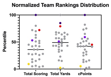
Figure 2 – The normalized distribution of team rankings with the Ravens (dark purple), Buccaneers (red), Vikings (light purple), and Steelers (Gold) highlighted. The black bar represents the median team value.
Trending in the other direction, the Vikings were around the median in number of total yards and around 50% for total scoring but were the 6th best offense by cPoints. On the bottom end, unfortunately the Steelers offense without Ben Roethlisberger was consistently bad, ranking 27th and 30th in total points and yards and 29th in cPoints. Importantly, while they did rank two spots above the Bengals in cPoints the normalized distribution shows there was effectively minimal difference between the four worst offenses last year (Steelers, Bengals, Jets, and Bears) and a meaningful gap to the 5th worst team of nearly 10%.
Other teams which showed large differences between cPoints and total scoring and yards included the: Patriots (down 10 spots for scoring and down 2 spots for yards), the Texans (up 7 for scoring and up 6 for yards), Colts (up 5 for scoring and up 13 for yards), and Panthers (down 7 for scoring and down 8 for yards).
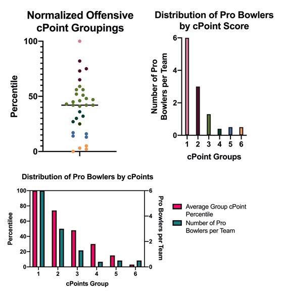
Figure 3 – Grouping of teams by offensive cPoints and its relationship to the number of offensive pro bowlers
Focusing on the grouping of offensive cPoint values, for the bottom four teams, I manually grouped the teams by cPoint scores (see Figure 3). The Ravens solely occupy the smallest group, while 14 teams occupy the largest (see Table 3), which would make sense given it falls near the middle of the distribution. Interestingly, this grouping also does somewhat correspond with the number of Pro Bowl players (prior to alternates being named) per team in the groups. The teams outside the top 3 in groups (bottom 13/32 teams) unsurprisingly on average had barely any pro bowlers. There was some interesting variation in the teams. Three of the teams in group 3 (Cardinals, Rams, and Patriots) did not have a Pro Bowl player following alternates, but the Browns and the Steelers (groups 4 and 6 respectively) had 2 players. While name recognition is well-known to play a role in Pro Bowl selections, for the Steelers the number of Pro Bowlers can also be looked at as the artifact of a team which was ready to make some waves prior to losing Ben Roethlisberger for the season.
Overall, offensive cPoints attempts to understand how, if we correct the offensive scoring and performance based on where the offenses got onto the field and what their outcomes were, our perspectives on who the best offenses in the league were. While the Ravens and the Chiefs were not surprising as the top two teams, it may have been more surprising to see the Cowboys (3rd), 49ers (5th), Vikings (6th), and Titans (8th). How did the Steelers get to 8 wins while being one of the worst offenses in the league? How did the Patriots with the median cPoints offense get to 12 wins? Both teams had fantastic defenses which will be the focus of the next article on cPoints, where I will conduct the opposite analysis focusing on defensive performance.
Table 3 – cPoint Grouping and Offensive Pro Bowlers (before alternates)
| Team | Normalized cPoints | cPoint Grouping | Offensive Pro Bowlers |
| Baltimore Ravens | 100% | 1 | 6 |
| Kansas City Chiefs | 82% | 2 | 3 |
| Dallas Cowboys | 75% | 2 | 4 |
| New Orleans Saints | 73% | 2 | 3 |
| San Francisco 49ers | 65% | 2 | 2 |
| Minnesota Vikings | 59% | 3 | 1 |
| Houston Texans | 56% | 3 | 3 |
| Tennessee Titans | 56% | 3 | 1 |
| Atlanta Falcons | 52% | 3 | 1 |
| Arizona Cardinals | 51% | 3 | 0 |
| Seattle Seahawks | 48% | 3 | 1 |
| Indianapolis Colts | 47% | 3 | 1 |
| Philadelphia Eagles | 46% | 3 | 3 |
| Tampa Bay Buccaneers | 45% | 3 | 2 |
| Green Bay Packers | 43% | 3 | 2 |
| Los Angeles Rams | 42% | 3 | 0 |
| New England Patriots | 42% | 3 | 0 |
| Oakland Raiders | 42% | 3 | 2 |
| Los Angeles Chargers | 41% | 3 | 1 |
| Detroit Lions | 36% | 4 | 0 |
| Cleveland Browns | 32% | 4 | 2 |
| New York Giants | 30% | 4 | 0 |
| Buffalo Bills | 27% | 4 | 0 |
| Denver Broncos | 25% | 4 | 0 |
| Miami Dolphins | 17% | 5 | 0 |
| Jacksonville Jaguars | 16% | 5 | 0 |
| Carolina Panthers | 14% | 5 | 1 |
| Washington Football Team | 13% | 5 | 1 |
| Pittsburgh Steelers | 5% | 6 | 2 |
| Chicago Bears | 3% | 6 | 0 |
| Cincinnati Bengals | 2% | 6 | 0 |
| New York Jets | 0% | 6 | 0 |
Methods of Calculating cPoints
Since offenses have several more outcomes than kickers, it may have been predictable that the calculation of cPoints was slightly more complex in this edition. As shown below, offensive cPoints were derived from three values: adjusted points scored (points scored with adjustments for field goal distance and safeties), expected points (from Figure 1), and deduction points (based on the expected field position data and expected punt/kick returns). Another way to look at expected vs. deducted points is that expected points are the points which the defense and special teams earned for the offense, for it to have the opportunity to start on that location on the field. The deduction points are the points that the offense is giving to the defense and special teams because of how they ended the drive.
The adjusted points were calculated for all drives that started outside overtime, the last 2 minutes of the half, or ended with the end of the half/game. Touchdowns remained at 7 points, field goals regardless of success were given their assigned expected value from the previous article on kicking, and safeties were assigned a -2 value since they give 2 points to the opposing team. The expected points were based on the regressed values (lines in Figure 1) mentioned earlier in the article.
The deduction points were taken based on setting a baseline value of the expected points from a kickoff (since scoring is the goal for offenses) as zero by subtracting the expected points from all other outcomes by this. Using Pro Football Reference, I found that the median and average return location code for kickoffs (excluding onside kicks) in 2019 was 15, corresponding to about an expected point value of 2. For punting (see Figure 4), using Pro Football Reference I again regressed the expected points for the opposing offense based on the starting punting location to find the “expected points for opposing offenses shown in the equation above”. Notably, this method allows the possibility for a team possibly having a negative deductive point if the expected points are below 2, which corresponds to the advantage for when the punting unit pins the opposing team deep in their own half of the field. For safeties I somewhat arbitrarily placed the expected points to be one location code closer (14). Finally, for turnovers, I used the expected points from the ending field position of the drive.
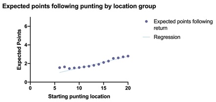
Figure 4 – Regressed expected points from punts based on starting location
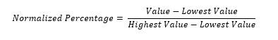
For normalizing the values between 0 and 100, I used the equation below. For example, to calculate the Steelers’ normalized percentage for cPoints, I put the difference between their value (-124.3) and the lowest recorded value (-139.3 by the Jets) in the numerator and the difference between the top recorded score (146.3 by the Ravens) and the lowest recorded value in the denominator. In this way, finding the normalized percentage for the top and bottom teams results in a value of 100% and 0% respectively.